Welcome
Welcome to the universal amplicon pipeline tutorial and setup workflow. This workflow helps you go from demultiplexed amplicon FASTQ files to a ready-to-run Snakemake configuration package.
The pipeline was designed around the 515F/926R universal primer pair, but it can be used with other amplicon primers provided the primer section is filled out correctly. It supports 16S and 18S reads, internal standards, and the metadata needed to generate the final files.
Use the sections below in order, then download the generated setup package when you are finished. The latest tested workflow is available in the pipeline repository on GitHub.
Why use a universal SSU rRNA primer set?
Metabarcoding using SSU rRNA as a marker gene is a powerful technique for profiling biological communities. Metabarcoding studies can be separated roughly into three groups:
- Studies of the “microbiome”—Bacteria and Archaea.
- Studies of microbial Eukarya, including phytoplankton and heterotrophic protists.
- Studies of macroscopic Eukarya, such as animals and plants.
The first group tends to use 16S SSU rRNA as a marker gene, while the second and third groups use 18S. PCR primer design has followed this division, with many primer sets targeting one group while discriminating against another.
However, 16S and 18S are, in evolutionary terms, the same molecule. SSU rRNA primers can therefore target both 16S and 18S in a single PCR assay. This is not two primer sets: one forward and one reverse primer amplify 16S from Archaea, Bacteria, chloroplasts, and mitochondria alongside eukaryotic nuclear 18S in the same tube.
That this is possible is remarkable. It shows that regions of the SSU rRNA molecule have remained sufficiently conserved across approximately 3.5 billion years of evolutionary history to amplify organisms as different as bacteria, chloroplasts, protists, and jellyfish.
Two example sequence pools
The first dataset comes from DNA extracted from 1 L of whole Pacific Ocean seawater filtered on a 0.2 µm Sterivex filter. It contains material ranging from prokaryotes and microbial eukaryotes to fragments, larvae, or propagules from animals.
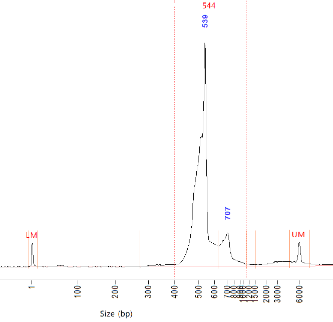
The second dataset comes from the same region of the Pacific Ocean, but larger organisms were concentrated with a net tow. Most of the DNA therefore comes from animals, protists, and other microeukaryotes.
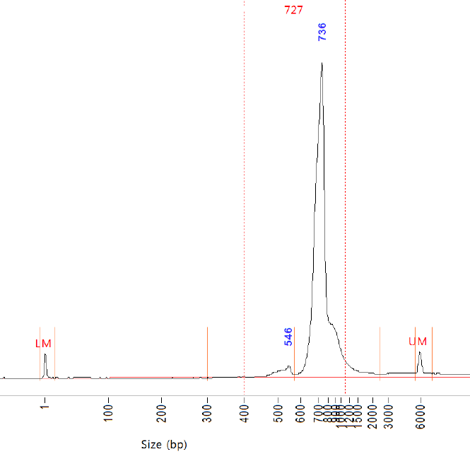
Why this pipeline is needed
One reason this approach has not been used more commonly is the mismatch between sequencing read lengths and amplicon lengths. The primers this pipeline was designed for bind at SSU rRNA coordinates 515 and 926 using E. coli as a reference. The resulting bacterial amplicon is approximately 411 bp, although its exact length varies among organisms. Archaeal amplicons are approximately the same length.
In Eukarya, the corresponding primer coordinates are 562 and 1150 in S. cerevisiae, producing an amplicon of approximately 588 bp. Although 18S length varies across evolutionary and ecological groups, eukaryotic amplicons are about 177 bp longer than prokaryotic amplicons on average.
Modern Illumina sequencing has a maximum paired-end read length of 300 bp, and low-quality bases—especially in the reverse read—must often be trimmed. The remaining forward and reverse reads usually overlap for 16S, but not for 18S. Most conventional amplicon pipelines require that overlap and consequently discard 18S reads from 515Y/926R data.
Based on an initial prototype by Mike Lee, Jesse McNichol refined a method for separating 16S and 18S reads in silico, and the pipeline grew from there. Yi-Chun Yeh, Melody Aleman, and Colette Fletcher-Hoppe have since made important contributions, many inspired by Jed Fuhrman’s ideas.
Repository and software setup
Install the required software, then enter your project name in the repository section below. This one name is used for the cloned directory, configuration, result filenames, and final Results-Export folder. Use a different name for each analysis so its configuration, logs, and results stay together.
Install the requirements
Install Git and Conda before continuing. The official Snakemake installation guide recommends a Conda-based installation. Administrator access is not normally required when Conda is installed in your user directory.
conda create --name snakemake --channel conda-forge --channel bioconda snakemake
conda activate snakemake
snakemake --version
Clone the pipeline repository
Choose a project name for this analysis. The generated command clones the pipeline from the public pipeline repository into a directory with that project name and then moves into it. You will not need to enter the project name again.
git clone https://github.com/Nwilliams96/515FY-926R-snakemake-NW-edits.git AMT29-analysis
cd AMT29-analysis
Config.yml
Fill these fields to generate the config/config.yml file used by the Snakemake workflow.
Database availability
Select each database family that is already complete and compatible with this pipeline. Leave an item unchecked when it needs to be downloaded or built. This allows, for example, an existing BBsplit and PR2 setup to be reused while only SILVA 144 is downloaded.
<name>_ng sample columns and are printed in the recovery-plot legend and correction-method labels.Internal standard information
Enter the copy number, genome length, and complete 16S sequence for every named standard.
BP, DR, and TT are prefilled from the common preset. If you rename one, its preset definition is cleared so it cannot be mistaken for the newly named standard.
18S pre-concatenation read-length controls
These lengths apply only to the 18S path, where R1 and R2 are trimmed before being concatenated. Paired 16S reads are no longer truncated to a fixed length; DADA2 receives their full post-primer-removal lengths.
16S DADA2 controls (paired reads)
The default 16S fixed truncation lengths are both 0, so DADA2 receives the complete post-primer-removal forward and reverse reads. Expected-error filtering, quality-score truncation, merging, and chimera removal still apply.
18S DADA2 controls (concatenated reads)
The 18S path concatenates trimmed R1 and R2 and then runs single-end DADA2, so it has no paired-read overlap setting.
Primer sequences
Enter the primer sequences that are still attached to the raw reads. Cutadapt uses these values to identify and remove primers before BBsplit and DADA2.
QIIME 2 environment
Choose whether to use an existing QIIME 2 environment definition and provide its location. This environment runs DADA2, taxonomy classification, and QIIME 2 artifact processing. The supplied QIIME 2 2026.7 definition is compatible with the official SILVA 144 classifier used by the pipeline. The classifier assigns Domain through Genus; the pipeline then adds a provisional Species label only for an unambiguous exact SILVA 144 sequence match whose genus agrees with that assignment. Unmatched or ambiguous ASVs remain blank at Species.
Sample File
Enter the number of samples to create the table, then type directly or paste a block of cells copied from Excel, Google Sheets, or equivalent software.
sample and the internal-standard fields. Add, rename, or remove columns—including depth, latitude, and longitude—then apply the list. The chosen columns are preserved downstream and become filters in the HTML taxonomy report.No additional columns configured.
Upload requires only sample and the configured internal-standard amount columns. Optional uploaded columns are retained, and omitted optional columns are left blank.
Amplicon Molarities
The 515F/926R primer pair targets both 16S and nuclear 18S rRNA. Unfortunately, there is a bias against 18S sequences when 16S and 18S sequences are mixed. This is because the 16S and 18S amplicons have different lengths (see the figures in the preamble) and are therefore sequenced at different rates, with a bias toward the shorter amplicons.
To correct for this, fill out this section of the configuration with the amounts of 16S and 18S molecules in the starting pool. These values can be obtained by running the pool on a TapeStation or Bioanalyzer, which most sequencing cores perform as part of quality control. The pipeline treats these values as the starting ratio, then calculates the ratio observed on the sequencing platform from the final 16S and 18S read counts. It uses the difference to increase the estimated 18S abundance and decrease the estimated 16S abundance accordingly.
Export
Once everything is filled in, export the package you can upload into the Snakemake directory.
config/
  README.md
  config.yml
  samples.tsv
  prok_and_euk_SSU_amplicon_molarities.tsv
  internal_stds.tsv  # included when internal standards are enabled
  schemas/
    config.schema.yml
    samples.schema.yml
  setup-scripts/
    setup-analysis-dir.sh
Your package will contain one complete config/ folder, including the README, schemas, and setup script.
username@hostname:/full/path/. You can also enter a local directory.scp ~/Downloads/AMT29-analysis-config.zip <OUTPUT_DESTINATION>
If you prefer a graphical file-transfer program, upload the ZIP to the same project directory using Cyberduck or FileZilla. Connect with SFTP using the hostname and login details supplied by your institution or server administrator.
config/ directory and the second refreshes every extracted config-file timestamp to prevent clock-skew errors on the compute system.unzip AMT29-analysis-config.zip
find config -type f -exec touch {} +
Run the pipeline
Once you have downloaded the configuration package, transferred it to the cloned project, and extracted it
so that the config/ directory is in the main project folder, activate the Snakemake environment
and run the included run_snakemake.sh script.
conda activate snakemake
bash run_snakemake.sh
The included script is intentionally minimal. Depending on your HPC system, you may need to add the appropriate
executor and resource allocation settings, such as jobs, CPUs, memory, runtime, account, or partition. The script
uses the shared conda_envs_dir from config/config.yml; existing matching environments are
reused automatically, and only missing or changed environments are created.
<project-name>-Results-Export/ folder. Its project-specific name prevents downloads from different runs being confused. It contains the formatted data tables, phylum and order summaries, and the self-contained HTML report.AMT29-analysis-Results-Export/AMT29.pipeline-report.html
Explore your ASV in GRUMP
If you used this pipeline with the same 515FY–926R primers and the same forward and reverse trim lengths used for GRUMP, you can copy an ASV hash from your results and search for it in the GRUMP Explorer. The explorer will show the ASV’s distribution across GRUMP samples.
Search an ASV hash in GRUMP